SDSS-II/SNLS3 Joint Light-curve Analysis
Table of Contents
This page contains links to data associated with the SDSS-II/SNLS3 Joint Light-Curve Analysis (Betoule et al. 2014, submitted to A&A).
The release consists in:
- The end products of the analysis and a C++ code to compute the likelihood of this data associated to a cosmological model. The code enables both evaluations of the complete likelihood, and fast evaluations of an approximate likelihood (see Betoule et al. 2014, Appendix E).
- The version 2.4 of the SALT2 light-curve model used for the analysis plus 200 random realizations usable for the propogation of model uncertainties.
- The exact set of Supernovae light-curves used in the analysis.
We also deliver presentation material.
Since March 2014, the JLA likelihood plugin is included in the official release of cosmomc. For older versions, the plugin is still available (see below: Installation of the cosmomc plugin).
To analyze the JLA sample with SNANA, see $SNDATA_ROOT/sample_input_files/JLA2014/AAA_README.
1 Release history
V1 (January 2014, paper submitted):
First arxiv version.
V2 (March 2014):
Same as v1 with additionnal information (R.A., Dec. and bias correction) in the file of light-curve parameters.
V3 (April 2014, paper accepted):
Same as v2 with the addition of a C++ likelihood code in an independant archive (jla_likelihood_v3.tgz).
V4 (June 2014):
Second arxiv version:
- Add the compressed version of the JLA likelihood (see Betoule et al. 2014, Appendix E)
- Make the C++ likelihood code (jla_likelihood_v4.tgz) the main product.
V5 (March 2015):
Correction of the C_stat.fits matrix (from archive file covmat_v4.tgz).
Previous to this release, the matrix contained in C_stat.fits was not the covariance matrix of light-curve parameters but a modified matrix, which, in particular was not positive. Off-diagonal entries of the \(C_{stat}\) matrix had been symetrized, the way the cosmomc plugin expect covariances between 2 different parameters to be given (as in the data/jla_*_covmatrix.dat files). As an exemple, the entry corresponding to \(cov(x_{1i}, c_j)\) with \(i \ne j\) contained instead \(0.5 \left[cov(x_{1i}, c_j) + cov(x_{1j}, c_i) \right]\).
It is important to note that this has no impact on the computation of the covariance of distance modulii and thus no impact in cosmological fits because both terms indeed play symetric roles there.
V6 (March 2015):
Change the presentation of the covmat tarball (see Error decomposition below) to match the presentation of uncertainties given in the paper.
2 Installation of the C++ likelihood code
The JLA C++ code and data are available from a single archive: jla_likelihood_v6.tgz. The code prerequisites working implementation of LAPACK and BLAS. To compile the static library edit the provided makefile to suit your local environment and do:
make
You may also need to adapt the name of lapack routines in jla.cc to match the convention of your fortran compiler.
The compilation of the provided example test depends on the CLASS CMB code for background computation. To compile this example fill the makefile with the path to your local class installation and type:
make test_jla
Running this test should perform an evaluation of both the complete and approximate JLA Chi2 for the best-fit LCDM model. The expected result is approximately \(-2 \log L = 682.9\) for the complete likelihood and \(-2 \log L = 33.62\) for the compressed approximate likelihood.
Light-curve parameters are given in file data/jla_lcparams.txt.
The columns are:
name: name of the SN
zcmb: CMB frame redshift (including peculiar velocity corrections for
      nearby supernova based on the models of M.J. Hudson)
zhel: Heliocentric redshift (note both zcmb and zhel are needed
      to compute the luminosity distance)
dz: redshift error (no longer used by the plugin)
mb: B band peak magnitude
dmb: Error in mb (includes contributions from intrinsic dispersion,
     lensing, and redshift uncertainty)
x1: SALT2 shape parameter
dx1: Error in shape parameter
colour: Colour parameter
dcolour: Error in colour
3rdvar: In these files, the log_10 host stellar mass
d3rdvar: Error in 3rdvar
tmax: Date of peak brightness (mjd)
dtmax: Error in tmax
cov_m_s: The covariance between mb and x1
cov_m_c: The covariance between mb and colour
cov_s_c: The covariance between x1 and colour
set: A number indicating which sample this SN belongs to, with
   1 - SNLS, 2 - SDSS, 3 - low-z, 4 - Riess HST
ra: Right Ascension in degree (J2000)
dec: Declination in degree (J2000)
biascor: The correction for analysis bias applied to measured magnitudes
	 (this correction is already applied to mb, original measurements
	  can be obtained by subtracting this term to mb)
Installation of the cosmomc plugin
Since March 2014, the JLA likelihood plugin is included in the official release of cosmomc. For older cosmomc versions, the original plugin is still available: jla_cosmo_v2.tgz.
Untar the archive and copy the following files to the corresponding cosmomc directory:
- source/supernovae_JLA.f90
- data/jla.dataset
- data/JLA.paramnames
- data/jla_*
Add the JLA likelihood in source/supernovae.f90:
use JLA
...
call JLALikelihood_Add(LikeList, Ini)
Modify the "SUPERNOVAE =" line of the cosmomc source/Makefile line to compile the JLA likelihood:
SUPERNOVAE = supernovae_Union2.o supernovae_SNLS.o supernovae_JLA.o
Depending on your cosmomc installation, you may obtain the same result by extracting directly the archive in your cosmomc directory.
3 SALT2 model
Version 2.4 of the SALT2 code, is available from the SALT2 home page. The corresponding data, including the model trained on the JLA training sample, and the description of instruments involved in the cosmology sample can be downloaded here: salt2-4_data.tgz (md5:af829c7f177c6037adcbe0a89360464a).
With this model, the fit of the lightcurves of SNLS 03D4ag (see Recalibrated light-curves in native SALT2 format) should return:
BEGIN_OF_FITPARAMS Salt2Model
DayMax 52830.9312582 0.0955792582608
Redshift 0.285 0 F
Color -0.0851965244364 0.0234763445429
X0 5.65786629794e-05 1.52744999131e-06
X1 0.937399343815 0.104657850633
RestFrameMag_0_B 21.2581394711 0.0292572971214
CovColorColor 0.000551138753097 -1
CovColorDayMax -0.00012040087613 -1
CovColorRestFrameMag_0_B 0.000524478290388 -1
CovColorX0 -2.73917683701e-08 -1
CovColorX1 -0.000243030505277 -1
CovDayMaxDayMax 0.00913539460969 -1
CovDayMaxRestFrameMag_0_B 0.000131399790871 -1
CovDayMaxX0 -6.85109541277e-09 -1
CovDayMaxX1 0.00179671536042 -1
CovRestFrameMag_0_BX0 -4.46890539999e-08 -1
CovRestFrameMag_0_BX1 0.00100854829146 -1
CovX0X0 2.33310347595e-12 -1
CovX0X1 -5.26149351948e-08 -1
CovX1X1 0.0109532656992 -1
END_OF_FITPARAMS Salt2Model
Note: This value of msb is different from the value published in Betoule et al. 2014 by -0.0012 because of malmquist bias correction.
4 Error propagation
Error decomposition
We deliver separate covariances matrices following the decomposition of the error on light-curve parameters proposed in Betoule et al. 2014, Eq. 11. The ordering of the \(3 \times N_{\rm SN} = 2220\) vector of light-curve parameters is: \[ \vec \eta = (m^\star_1, {X_1}_1, C_1, \cdots, m^\star_{N_{\rm SN}}, {X_1}_{N_{\rm SN}}, C_{N_{\rm SN}}). \] The covariance matrix of this vector can be assembled as: \[ C_{\vec \eta} = C_{\rm stat} + C_{\rm cal} + C_{\rm model} + C_{\rm bias} + C_{\rm host} + C_{\rm dust} + C_{\rm pecvel} + C_{\rm nonIa} \] with:
- \(C_{\rm stat} \): statistical uncertainty (including the statistical uncertainty of the SALT2 Model, but without \(\sigma_{\rm coh}\) and \(\sigma_{lens}\) of Eq. 13)
- \(C_{\rm cal} \): calibration uncertainty
- \(C_{\rm model} \): systematic uncertainty on the model (See Mosher et al. 2014)
- \(C_{\rm bias} \): uncertainty on the bias correction
- \(C_{\rm host} \): uncertainty on the fonctionnal form of the luminosity-host mass relation.
- \(C_{\rm dust} \): uncertainty on the Milky Way dust column density
- \(C_{\rm pecvel}\): uncertainty on the peculiar velocity correction (Systematic only: does not include the \(\sigma_z\) term of Eq. 13.)
- \(C_{\rm nonIa} \): potential contamination by non-Ia.
Given the values of \(\alpha\) and \(\beta\) parameters, the covariance matrix of distance modulii can be assembled following Eq. 13 of Betoule et al. (2014):
\[ C = A C_{\vec \eta} A^T + {\rm diag}\left(\frac{5\sigma_z}{z\log 10}\right)^2 + {\rm diag}(\sigma_\text{lens}^2 ) + {\rm diag}(\sigma_\text{coh}^2) \,. \]
The \(3N_{\rm SN}\times 3N_{\rm SN} = 2220\times2220\) matrices and the \(\sigma_{coh}\) and \(\sigma_{lens}\) vectors are provided in covmat_v6.tgz. A sample python script is provided to illustrate computation of \(C\) from the given products.
SALT2 light-curve model uncertainties
Photometric calibration uncertainties in the training data sample affect the recovered SALT2 model. The resulting error in turn affects coherently all the light-curve fitted with this model. We emphasize that *assuming a perfect calibration of the model when fitting for supernovae can result in a serious underestimation of the actual uncertainty*.
In order to enable the propagation of uncertainties associated with the use of the SALT2 model, we release a set of 200 random realizations of the model, drawn according to the estimate of calibration uncertainties affecting the JLA training sample:
To obtain an estimate of the covariance of fit parameters: A possibility is to fit a set of SNe light-curves with each random realization and estimate the covariance of
5 Recalibrated light-curves in native SALT2 format
Light curves of SN includes in the cosmology sample: jla_light_curves.tgz (md5:14f402041003661d284ac18dbcc7ec24).
It includes:
- the recalibrated SNLS3 light curve (lc-??D??.list)
- the recalibrated SDSS-II light-curves (lc-SDSS*.list, subsample of http://sdssdp62.fnal.gov/sdsssn/DataRelease/index.html)
- Nearby and HST light-curves from the C11 compilation (lc-sn*.list and lc-name.list, available from https://tspace.library.utoronto.ca/snls/)
Six SNe (sn2005hc, sn2005ir, sn2006nz, sn2006oa, sn2006ob, sn2006on) are in common with SDSS and either CfAIII or CSP. The light-curve file contains a merge of all available photometry.
6 Presentation material
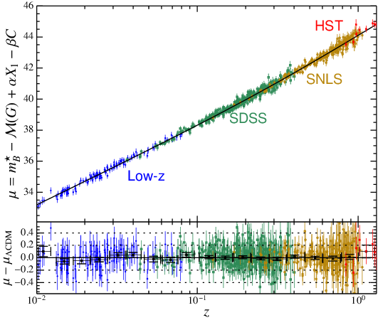
Figure 1: JLA Hubble diagram
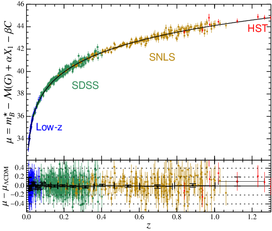
Figure 2: Alternative JLA Hubble diagram (linear x axis)
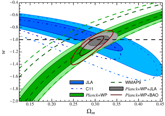
Figure 3: Flat w-CDM fit parameters
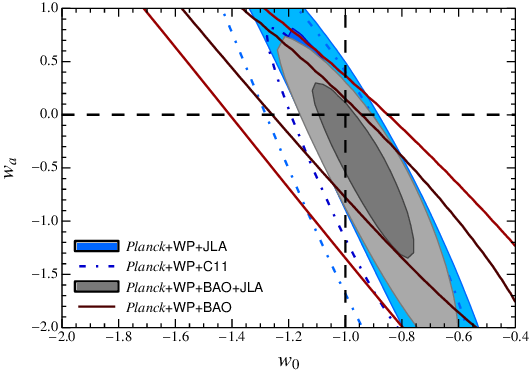
Figure 4: Flat wz-CDM fit parameters
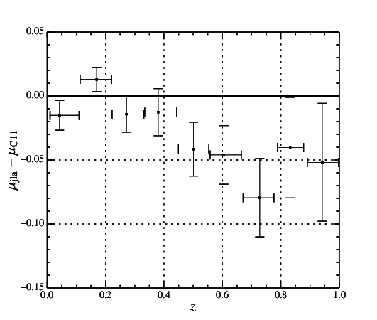
Figure 5: Difference in distance modulus between the JLA and Conley et al. (2011) hubble diagrams